Generally, implementing an OBDA architecture atop Big Data raises three challenges:

• Query translation. SPARQL queries must be translated into the query language of each of the respective data sources. A generic and dynamic translation between data models is challenging (even impossible in some cases e.g., join operations are unsupported in Cassandra and MongoDB).
• Federated Query Execution. In Big Data scenarios it is common to have non-selective queries with large intermediate results, so joining or aggregation cannot be performed on a single node, but only distributed across a cluster.
• Data silos. Data coming from various sources can be connected to generate new insights, but it may not be readily ‘joinable’ (cf. definition below).

To target the aforementioned challenges we have built Squerall, an extensible framework for querying Data Lakes.

• It allows ad hoc querying of large and heterogeneous data sources virtually without any data transformation or materialization.
• It allows the distributed query execution, in particular the joining of disparate heterogeneous sources.
• It enables users to declare query-time transformations for altering join keys and thus making data joinable.
• Squerall integrates the state-of-the-art Big Data engines Apache Spark and Presto with the semantic technologies RML and FnO.

System Overview

Squerall General Architecture

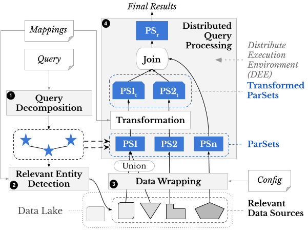
Squerall consists of four main components (see numbered boxes in the figure above). Because of Squerall extensible design, also for clarity, we here use the generic ParSets and DEE concepts instead of Squerall’s underlying equivalent concrete terms, which differ from engine to engine. ParSet, from Parallel dataSet, is a data structure that can be distributed and operated on in parallel; it follows certain data model, like tables in tabular databases, graph in graph databases, or a document in a document database. DEE, from Distributed Execution Environment, is the shared physical space where ParSets can be transformed, aggregated and joined together.

The architecture accepts three user inputs (refer to Squerall Basics for more details):

• Mappings: it contains association between data source entities and attributes (eg table and column in a tabular database or collection and document in a document database) to ontology properties and classes.
• Config: it contains the access information needed to connect to the heterogeneous data sources, e.g., username, password, or cluster setting, e.g., hosts, ports, cluster name, etc.
• Query: a query in SPARQL query language.

The fours components of the architecture are described as follows:

(1) Query Decomposor. This component is commonly found in OBDA and query federation systems. It decomposes the query’s Basic Graph Pattern (BGP, conjunctive set of triple patterns in the where clause) into a set of star-shaped sub-BGPs, where each sub-BGP contains all the triple patterns sharing the same subject variable. We refer to these sub-BGPs as stars for brevity; (see below figure left, stars are shown in distinct colored boxes).

(2) Relevant Entity Extractor. For every extracted star, this component looks in the Mappings for entities that have attributes mappings to each of the properties of the star. Such entities are relevant to the star.

(3) Data Wrapper. In the classical OBDA, SPARQL query has to be translated to the query language of the relevant data sources. This is in practice hard to achieve in the highly heterogeneous Data Lake settings. Therefore, numerous recent publications advocated for the use of an intermediate query language. In our case, the intermediate query language is DEE’s query language, dictated by its internal data structure. The Data Wrapper generates data in POA’s data structure at query-time, which allows for the parallel execution of expensive operations, e.g., join. There must exist wrappers to convert data entities from the source to DEE’s data structure, either fully, or partially if parts of the data can be pushed down to the original source. Each identified star from step (1) will generate exactly one ParSet. If more than an entity are relevant, the ParSet is formed as a union. An auxiliary user input Config is used to guide the conversion process, e.g., authentication, or deployment specifications.

(4) Distributed Query Processor. Finally, ParSets are joined together forming the final results. ParSets in the DEE can undergo any query operation, e.g., selection, aggregation, ordering, etc. However, since our focus is on querying multiple data sources, the emphasis is on the join operation. Joins between stars translate into joins between ParSets (figure below phase I). Next, ParSet pairs are all iteratively joined to form the Results ParSet (figure below phase II) . In short, extracted join pairs are initially stored in an array. After the first pair is joined, it iterates through each remaining pair to attempt further joins or, else, add to a queue . Next, the queue is similarly iterated, when a pair is joined, it is unqueued. The algorithm completes when the queue is empty. As the Results ParSet is a ParSet, it can also undergo query operations. The join capability of ParSets in the DEE replaces the lack of the join common in many NoSQL databases, e.g., Cassandra, MongoDB. Sometimes ParSets cannot be readily joined due to a syntactic mismatch between attribute values. Squerall allows users to declare Transformations, which are atomic operations applied to textual or numeral values.

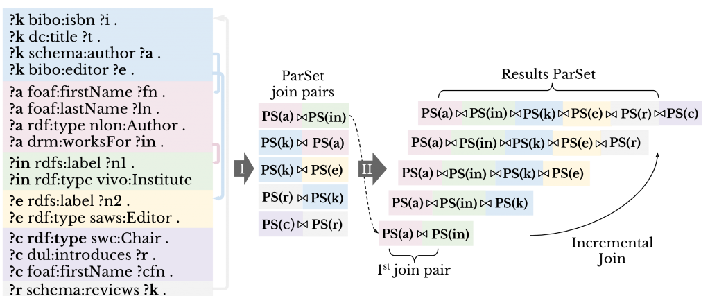
From query to ParSets to joins between ParSets

Squerall has two query engine implementations using Apache Spark and Presto. For Spark, ParSets are represented by DataFrames and joins between ParSets are translated into joins between DataFrames. Presto accepts only SQL queries, so ParSets are represented by SQL SELECT sub-queries, and joins between ParSets are represented by join between SELECT sub-queries. Similarly, operations on ParSets derived from the SPARQL query are translated into equivalent SQL functions in Spark and SQL operations in Presto.

Evaluation

We evaluate Squerall performance when using Berlin Benchmark (BSBM) with three scales (0,5M, 1,5M, 5M products), nine adapted queries and five data sources (Cassandra, MongoDB, Parquet, CSV, MySQL) populated from BSBM generated data. The experiments were run in a cluster of three machines each having DELL PowerEdge R815, 2x AMD Opteron 6376 (16 cores) CPU and 256GB RAM.

We compare the query execution time between Spark-based Squerall vs Presto-based Squerall. The results, shown in the below figure suggest that Presto-based Squerall is faster in the majority of queries than Spark-based Squerall.

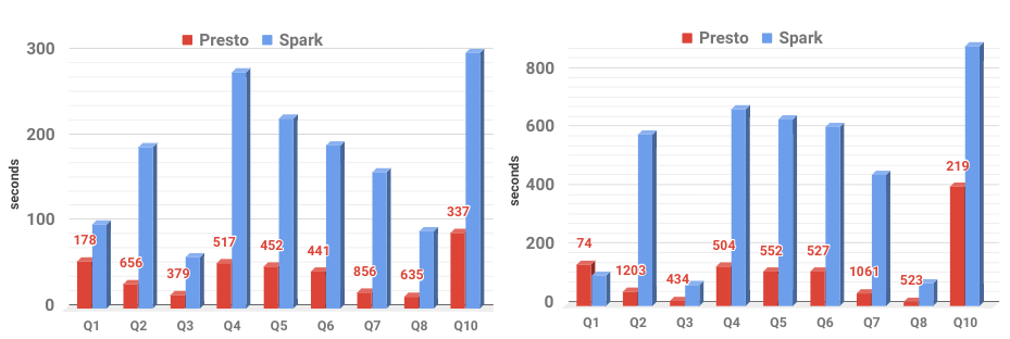
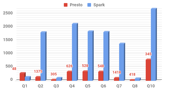
Figure: Query Execution Time of the three scales, 0,5M top left, 1,5M top right and 5M bottom. The numbers on top of Presto bars show percentage of Spark’s execution time to Presto’s, e.g., 178 means that Presto is 178% faster than Spark.

We also record the time taken by the sub-phases of the query execution. Results suggest that Query Analysis and Relevant Source Detection phases have a minimum contribution to the overall query execution process, and that the actual Query Execution by Spark/Presto is what dominates the process.

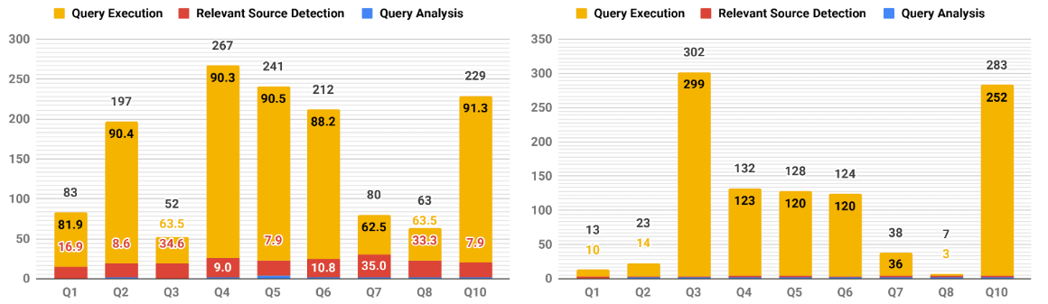
Query Execution Time breakdown into its sub-phases: Query Analysis, Relevant Source Detection and Query Execution.

In order to evaluate the ratio between query execution and data size scales, we plot the query execution times of the three scales into one graph.

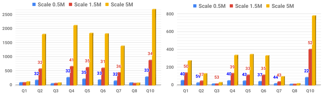
Scalability of Query Execution Time versus Data Size. Spark-based Squerall in the left and Presto-based in the right.

Publications

For further reading and full details, we refer readers to the following publications:

• Squerall: Virtual Ontology-Based Access to Heterogeneous and Large Data Sources
• Uniform Access to Multiform Data Lakes using Semantic Technologies
• Querying Data Lakes using Spark and Presto
• How to feed the Squerall with RDF and other data nuts?