In recent years, our information society has reached the stage where it produces billions of data records, amounting to multiple quintillion of bytes, on a daily basis. Extraction, cleansing, enrichment and refinement of information are key to fuel value-adding processes, such as analytics as a premise for decision making. For a better representation and capable of extracting desired information there is an effort of better representing such a large amount of data (e.g. metadata). The efforts have been made constantly. The most prominent and promising effort is the W3C consortium with encouraging Resource Description Framework (RDF) as a common data representation and vocabularies (e.g. RDFS, OWL) a way to include meta-information about the data. These data and meta-data can be further processed and analyzed using the de-facto query language for RDF data, SPARQL.
SPARQL serve as a standard query language for manipulating and retrieving RDF data. Querying RDF data becomes challenging when the size of the data increases. Recently, many distributed RDF systems capable of evaluating SPARQL queries have been proposed and developed.
Nevertheless, these engines lack one important information derived from the knowledge, RDF terms. RDF terms include information about a statement such as a language, typed literals and blank nodes which are omitted from most of the engines.
To cover this spectrum requires a specialized system which is capable of constructing an efficient SPARQL query engine. Doing so comes with several challenges. First and foremost, recently the RDF data is increasing drastically. Just as a record, today we count more than 10,0000 datasets available online represent using the Semantic Web standards. This number is increasing daily including many other (e.g Ethereum dataset) datasets available at the organization premises. In addition, being able to query this large amount of data in an efficient and faster way is a requirement from most of the SPARQL evaluators.
To overcome these challenges, in this paper, we propose Sparklify: a scalable software component for efficient evaluation of SPARQL queries over distributed RDF datasets. The conceptual foundation is the application of ontology-based data access (OBDA) tooling, specifically SPARQL-to-SQL rewriting, for translating SPARQL queries into Spark executable code. We demonstrate our approach using Sparqlify, which has been used in the LinkedGeoData community project to serve more than 30 billion triples on-the-fly from a relational OpenStreetMap database.
System Overview
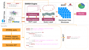
Fig. 1. Sparklify Architecture Overview
The overall system architecture is shown in Fig.1. It consists of four main components: Data Model, Mappings, Query Translator and Query Evaluator.
In the following, each component is discussed in details.
- Data Model — SANSA comes with different data structures and different partitioning strategies. We model and store RDF graph following the concept of RDDs — a basic building blocks of the Spark Framework. RDDs are in-memory collections of records which are capable of operating in a parallel overall larger cluster. Sparklify makes use of SANSA bottom layer which corresponds with the extended vertical partitioning (VP) including RDF terms. This partition model is the most convenient storage model for fast processing of RDF datasets on top of HDFS.
Data Ingestion – RDF data first needs to be loaded into a large-scale storage that Spark can efficiently read from.We use Hadoop Distributed File-System (HDFS). Spark employ different data locality scheme in order to accomplish computations nearest to the desired data in HDFS, as a result avoiding i/o overhead.
Data Partition – VP approach in SANSA is designed to support extensible partitioning of RDF data. Instead of dealing with a single three-column table $(s, p, o)$, data is partitioned into multiple tables based on the used RDF predicates, RDF term types and literal datatypes. The first column of these tables is always a string representing the subject. The second column always represents the literal value as a Scala/Java datatype. Tables for storing literals with language tags have an additional third string column for the language tag. - Mappings/Views — After the RDF data has been partitioned using the extensible VP (as it has been described on \textit{step 2}) the relational-to-RDF mapping is performed. Sparqlify supports both the W3C standard R2RML sparqlification. The main entities defined with SML are view definitions. The actual view definition is declared by the Create View … As in the first line. The reminder of the view contains these parts : (1) the Form directive defines the logical table based on the partitioned table. (2) an RDF pattern is defined in the Construct block containing, URI, blank node or literals constants (e.g. ex:worksAt) and variables (e.g. ?emp, ?institute}). The With block map the variables used in the triple pattern via term constructor expressions. This constructor expressions refer to columns of the logical table.
- Query Translation — This process generates a SQL query from the SPARQL query using the bindings determined in the mapping/views phases. It walks through the SPARQL query using the Jena ARQ and generate the SPARQL Algebra Expression Tree (AET). Further, these AETs are normalized in order to eliminate the self joins. Finally, the SQL is generated using the bindings corresponding the views.
- Query Evaluator — The SQL query created as described in the previous section can now be evaluated directly into the Spark SQL engine. The result set of this SQL query is distributed data structure of Spark (e.g. DataFrame) which then is mapped into a SPARQL bindings. The result set can further used for analysis and visualization using the SANSA-Notebooks.
How to use it
The component is part of the SANSA Stack, therefore it comes as implicit of the SANSA. Below, we give one examples of the Sparklify approach which can be called using the SANSA API.
-
In this example, we use SANSA readers to build a dataset of RDD[Triple] called triples and then compute some of the quality metrics.
1234567891011import net.sansa_stack.rdf.spark.io._import net.sansa_stack.query.spark.query._import org.apache.jena.riot.Langval input = "hdfs://..."val lang = Lang.NTRIPLESval triples = spark.rdf(lang)(input)val sparqlQuery = "SELECT * WHERE {?s ?p ?o} LIMIT 10"val result = triples.sparql(sparqlQuery)Full example code: https://github.com/SANSA-Stack/SANSA-Examples/blob/develop/sansa-examples-spark/src/main/scala/net/sansa_stack/examples/spark/query/Sparqlify.scala
The Sparklify has been piped into the SANSA-Notebooks as well, therefore users can use it without many configurations beforehand. SANSA-Notebooks is developer-friendly access to SANSA, which provide a web-editor interface for using the SANSA functionality.
Full example code: https://github.com/SANSA-Stack/SANSA-Notebooks/wiki/Query-notebook#sparklify-example
Evaluation
The goal of Sparklify evaluation is to observe the impact of the extensible VP as well as analyzing its scalability when the size of the datset increases.
At the same time, we also want to measure the effect of using Sparqlify optimizer for improving query performance.
In the following, we present our experiments setting including the benchmarks used and server configurations.
-
We used two well-known SPARQL benchmarks for our evaluation. The Lehight University Benchmak (LUBM) v3.1 and Waterloo SPARQL Diversity Test Suite (WatDiv) v0.6.
Characteristics of the considered datasets are given in Table. 1.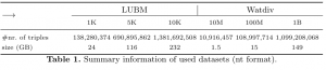
We implemented Sparklify using Spark-2.4.0, Scala 2.11.11, Java 8, and Sparqlify 0.8.3 and all the data were stored on the HDFS cluster using Hadoop 2.8.0.
All experiments were carried out on a commodity cluster of 7 nodes (1 master, 6 workers): Intel(R) Xeon(R) CPU E5-2620 v4 @ 2.10GHz (32 Cores), 128 GB RAM, 12 TB SATA RAID-5, connected via a Gigabit network.
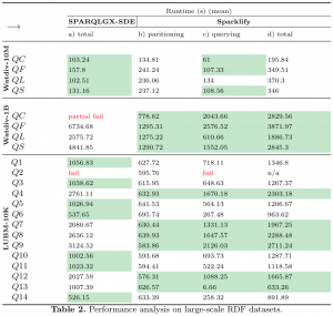
The experiments have been executed three times and the average runtime has been reported into the results. We evaluate Sparklify using the above datasets and compare it with the chosen state-of-the-art distributed SPARQL query evaluator.
We compare our approach with SPARQLGX‘s direct evaluator named SDE and report the loading time for partitioning and query execution time, see Table.2.
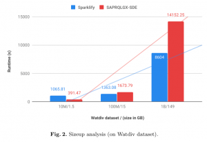
Size-up scalability analysis —To measure the performance of the data scalability (e.g. size-up) of both approaches, we run experiments on three different sizes of Watdiv (see Fig.2). We keep the number of nodes constant i.e 6 worker nodes and grow the size of the datasets to measure whether both approaches can deal with larger datasets. We see that the execution time for Sparklify grows linearly compared with SPARQLGX-SDE, which keeps staying as near-linear when the size of the datasets increases.
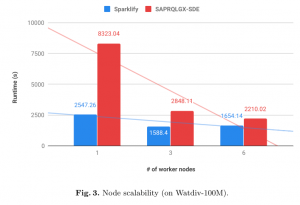
Node scalability analysis — To measure the node scalability of Sparklify, we vary the number of worker nodes. We vary them from 1, 3 to 6 worker nodes. Fig. 3 depict the speedup performance of both approaches run on Watdiv-100M datasaet when the number of worker nodes varies. We can see that as the number of nodes increases, the runtime cost for the Sparklify decrease linearly. The execution time for Sparklify decreases about 0.6 times (from 2547.26 seconds down to 1588.4 seconds) as worker nodes increase from one to three nodes. We see that the speedup stays constant when more worker nodes are added since the size of the data is not that large and the network overhead increases a little the runtime when it runs over six worker nodes. This imply that our approach is efficient up to three worker nodes for the Watdiv-100M (15GB) dataset. In another hand, SPARQLGX-SDE takes longer to evaluate the queries when running on one worker node but it improves when the number of worker nodes increases.